Steady and Transient Heat Conduction of a Large Uranium Plate
Purpose: Heat is an important design consideration in a multitude of industries that if left unaccounted for can cause anywhere from minor damage of components to catastrophic failure of critical systems. Although the Chernobyl disaster that occurred in 1986 was caused by human negligence, the resulting events that unfolded were the effects of thermal runaway. Knowing both the magnitude and direction of where heat is flowing at any given time allows the engineer to properly design around it and/or develop adequate cooling solutions. Heat and mass transfer problems introduced at the undergraduate level are typically only solvable analytically if they share both simple geometries and simple boundary conditions. Problems encountered in the real world are rarely this simplified, often requiring the engineer to use a software simulation package to perform a numerical method for a sufficiently accurate approximation. Software packages provide the engineer with a concrete answer as well as graphical insights to better communicate their findings. In the following example problems, I use ANSYS Mechanical to perform a thermal analysis.
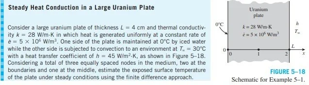
Problem taken from Cengel & Ghajar Heat and Mass Transfer: Fundamentals & Applications 5th ed.
136.04
The exposed surface temperature was determined to be 136.04 degrees Celsius by placing a temperature probe on the right wall.
Verification & Validation: A major issue with using software simulations is the ease of use and the ability to have cool looking graphics in the matter of seconds — but how do we add confidence to our results and increase certainty that we have correctly modeled the problem? The quickest way would be by intuitively looking at our results and using fundamental knowledge of the system modeled. In this case, the problem states the left side of the plate is maintained at 0 degrees. As can be seen by our results, the left side remains 0 degrees. Also, the top and bottom of the plate is perfectly insulated meaning no heat can flow between the boundary, and so the temperature gradient must remain zero along our y-axis. As can be seen in our results, temperature is only a function of x. Another way to verify the accuracy of our results would be to do a hand calculation, typically using a simpler geometry for a rough ballpark number. Thankfully this problem proves that simple geometry condition to be true that an analytical solution to the differential equation exists:

The three-dimensional heat conduction equation is reduced to one-direction as temperature varies in the x-direction only. Inputting x = 0.04m (40 mm) results in a T value of 136 degrees Celsius, further validating the model.
Conclusion: Although a simple problem with a function that exists, I thought this served as a great introduction to engineering software, properly setting boundary conditions, and utilizing the finite element method to solve heat transfer problems. At the very least, we are able to easily visualize the temperature gradient across the 40 mm uranium plate and better understand the temperature profile. A more accurate model can be acquired by refining the mesh and adding more nodes, but that comes at a cost of longer computing time. Below I solve the same problem but with a heat flow that changes over time (transient), and to my knowledge, a problem where an analytical solution is not readily available.
Problem taken from Cengel & Ghajar Heat and Mass Transfer: Fundamentals & Applications 5th ed.
143.9
The exposed surface temperature 2.5 mins after the start of cooling was determined to be 143.9 degrees Celsius by placing a temperature probe on the right wall and analyzing the data after 150 seconds.
Verification & Validation: Intuitively it makes sense that the temperature is decreasing over time, as the plate is being cooled. To solve this manually we could use a technique similar to the computer and resort to the finite difference method. The finite difference method is really only feasible through software as it requires deconstructing ordinary and partial differential equations into a system of linear equations that can be solved via matrix algebra. The book already provides the answer below, with the same answer received in ANSYS.

Answer taken from Cengel & Ghajar Heat and Mass Transfer: Fundamentals & Applications 5th ed.
Conclusion: ANSYS Mechanical is a fantastic finite element analysis tool to solve heat transfer problems. What used to take much longer in Excel/Python scripts has been replaced by ANSYS in the matter of minutes. It’s amazing how quickly it is able to solve an empathetically large number of equations simultaneously and provide the user with meaningful results. I think with such a low learning curve entry to jump in and start creating stunning visuals that the greatest difficulty in the software is conceptually understanding the problem and properly labelling the initial/boundary conditions.
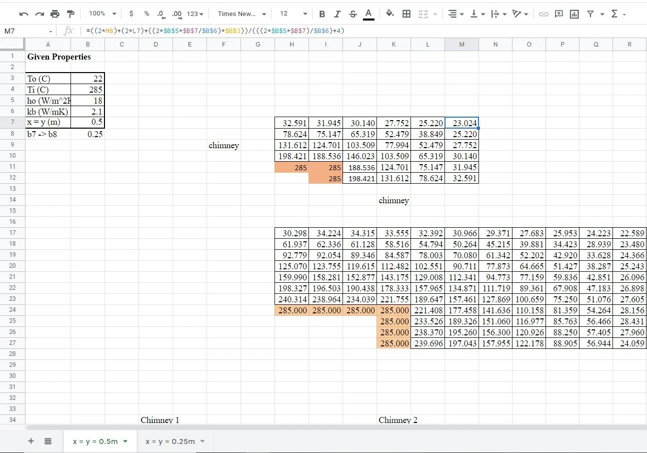
An absolute monster of a Google Sheets I created as an undergraduate student to solve Steady State Two-Dimensional Heat Conduction in a chimney using the Finite Difference Method

Development of the stiffness matrix. How ANSYS works under-the-hood to convert the differential equation into an algebraic system of equations solvable by the computer. [See Galerkin method for better detail (super cool)] (Credits to Prof. Bhaskaran (Cornell University))